How to run using cae¶

The plugins commands are available from within CAE as:

A toolbar, activate by Plug-ins ‣ Toolboxes ‣ Rollover
Menu items, in Plug-ins ‣ Rollover

Creating the rail¶

A basic rail is created with the command Create rail... rail_icon , opening the following form

rail_form

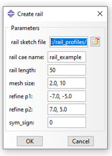
The following table describes the options

Parameter	Description
rail sketch file	The path to the rail sketch, see Creating a profile sketch and The data folder and how to specify paths
rail cae name	Name of the Abaqus Model Database (.cae) file to be created
rail length	The extrusion length of the rail
mesh size	The fine and coarse mesh size, separated by a comma
refine p1	The first point (x,y) defining the refine rectangle
refine p2	The second point defining the refine rectangle
sym_sign	If symmetry about the yz-plane is used, specify the x-direction (-1 or +1), pointing away from the material. Set to 0 if symmetry is not used.

This will create a rail part, which could look like the following

rail_basic

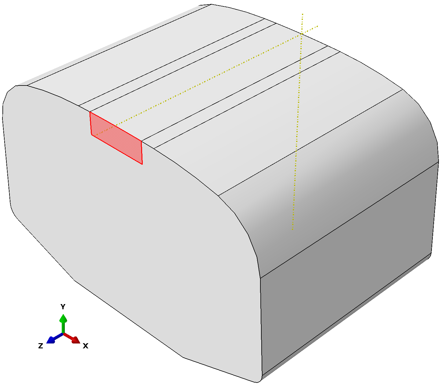
The red region marks the refine rectangle. This rectangle is used to create a cell by partitioning the rail by extrusion in the z-direction. The generated cell serves two purposes. Firstly, it controls where the fine mesh is used. Secondly, the external faces belonging to the cell, except the end faces with normal in the z-direction, make up the contact region.

The rail can now be modified to suit the needs of the simulation, e.g. changing the geometry, mesh and material definitions. The requirements on the rail are given in Modifying the basic rail. Note that the tool to make a TET mesh periodic is available as a plugin:

Plug-ins ‣ Rollover ‣ Tools ‣ Periodize mesh or on the Rollover toolbar: periodize_icon

Creating a wheel¶

A wheel is created with the command Create wheel... wheel_icon , opening the following form

wheel_form

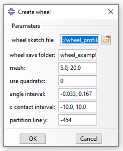
The following table describes the options

Parameter	Description
wheel sketch file	The path to the wheel sketch, see Creating a profile sketch and The data folder and how to specify paths
wheel save folder	Name of the folder in which the wheel super element files should be saved.
mesh	The fine and coarse mesh size, separated by comma
use quadratic	0 for linear elements, 1 for quadratic elements
angle interval	The angular interval in which to retain wheel nodes. Measured in radians around x, relative the negative y-axis.
x contact interval	The x-interval in which to retain wheel nodes.
partition line y	The y-coordinate (in the sketch, typically negative) outside which the fine mesh should be applied.

Upon pressing OK, a wheel substructure is calculated. This can take considerable time, especially for fine meshes. It is therefore recommended to test first with a bit coarser mesh. It is particularly the fine mesh size that determines the size, as this is used to determine the angular interval to mesh the wheel. For the default settings with a very coarse mesh, the full wheel mesh looks like

wheel_full

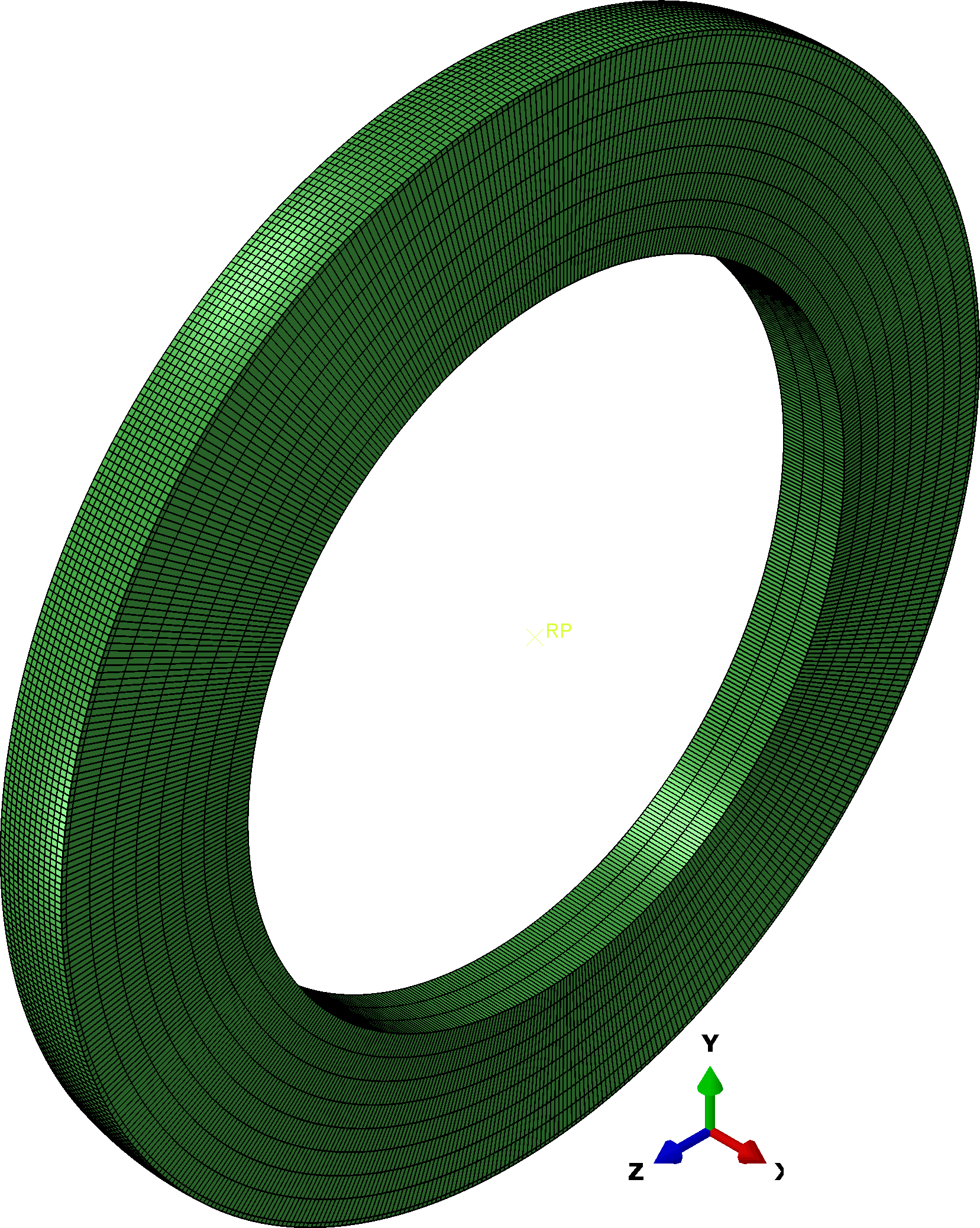
Note, however, that it is currently not supported to manually edit the wheel mesh. The motivation is that once the wheel only needs to be calculated once, and it is therefore not required to optimize the mesh.

Creating the simulation¶

A simulation is created with the command Create simulation... rollover_icon , opening the following form

rollover_form

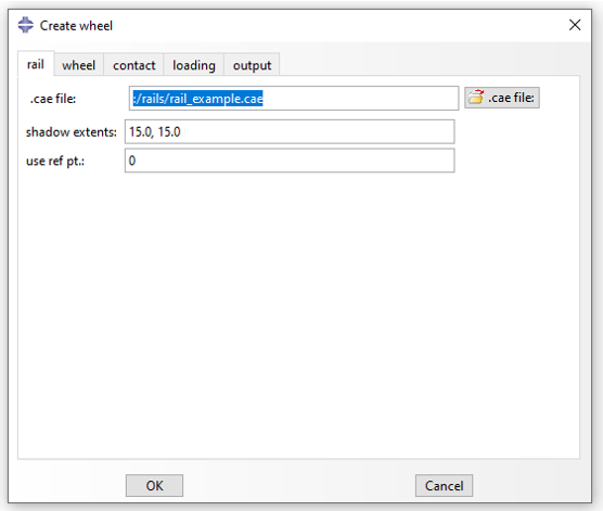
This form has multiple tabs, which are described by the following tables

Rail
.cae file	The path to the rail Abaqus Model Database file (.cae)
shadow extents	Name of the folder in which the wheel super element files should be saved.
use ref pt.

Wheel
folder	The folder containing the wheel super element files
translation	The vector (x,y,z) which the wheel should be translated on import. Initially, the wheel center is at (0,0,0). The rail sketch determines the (x,y) position of the rail, and it starts at z=0 and ends at z=L, where L is the rail length specified above.
use ref pt.	If rail extension should be used, a reference point is required. Otherwise, fewer constraints are added creating a slightly more efficient simulation. Set to 0 for no reference point, 1 otherwise.

Contact
friction coeff	The friction coefficient for the contact
contact stiff	The constant contact stiffness used (penalty method)

Loading
initial depression	How much to move the wheel control point in negative y-direction using displacement control, before switching to load control, in the first cycle
time inbetween	Which step time to use for the initial steps and the steps when mapping back the wheel in each cycle.
inbetween max incr	Maximum number of increments for the above steps.
rolling length	The rolling length, should match the rail length.
rolling radius	The rolling radius used to convert slip to rotation speed.
max increments	Maximum number of increments for one rolling step
min increments	Minimum number of increments for one rolling step
num cycles	Number of cycles to simulate. Please read Adding rolling cycles
cycles spec	The cycles for which a change in loading conditions are specified. Given as csv, matching “cycles spec”
wheel load	The force applied to the wheel control point in negative y-direction. Given as csv, matching “cycles spec”
speed	The linear speed for the wheel control point. Given as csv, matching “cycles spec”
slip	The wheel slip \(s\), such that \(\dot{\theta}_x = (1+s)\frac{v}{R}\) where \(\dot{\theta}_x\) is the wheel control point rotation speed around x, \(v\) is the speed and \(R\) is the “rolling radius” Given as csv, matching “cycles spec”
rail ext	The rail extension at the end of the rolling cycle, varying linearly to this value. Given as csv, matching “cycles spec”

Output
name	The name of the field output request to be created
set	The rail set name to take field output data for. Additionally, the names “FULL_MODEL” (both rail and wheel) and “WHEEL_RP” (wheel reference point) are supported.
variables	Which variables to output, comma separated, to find the correct variables, see the string created when setting up a field output request from within CAE.
frequency	How often (in terms of increments) to save data
cycle	How often (in terms of cycles) to save data. If e.g. 25 if specified, output will occur at cycle 1, 26, 51, and so on.

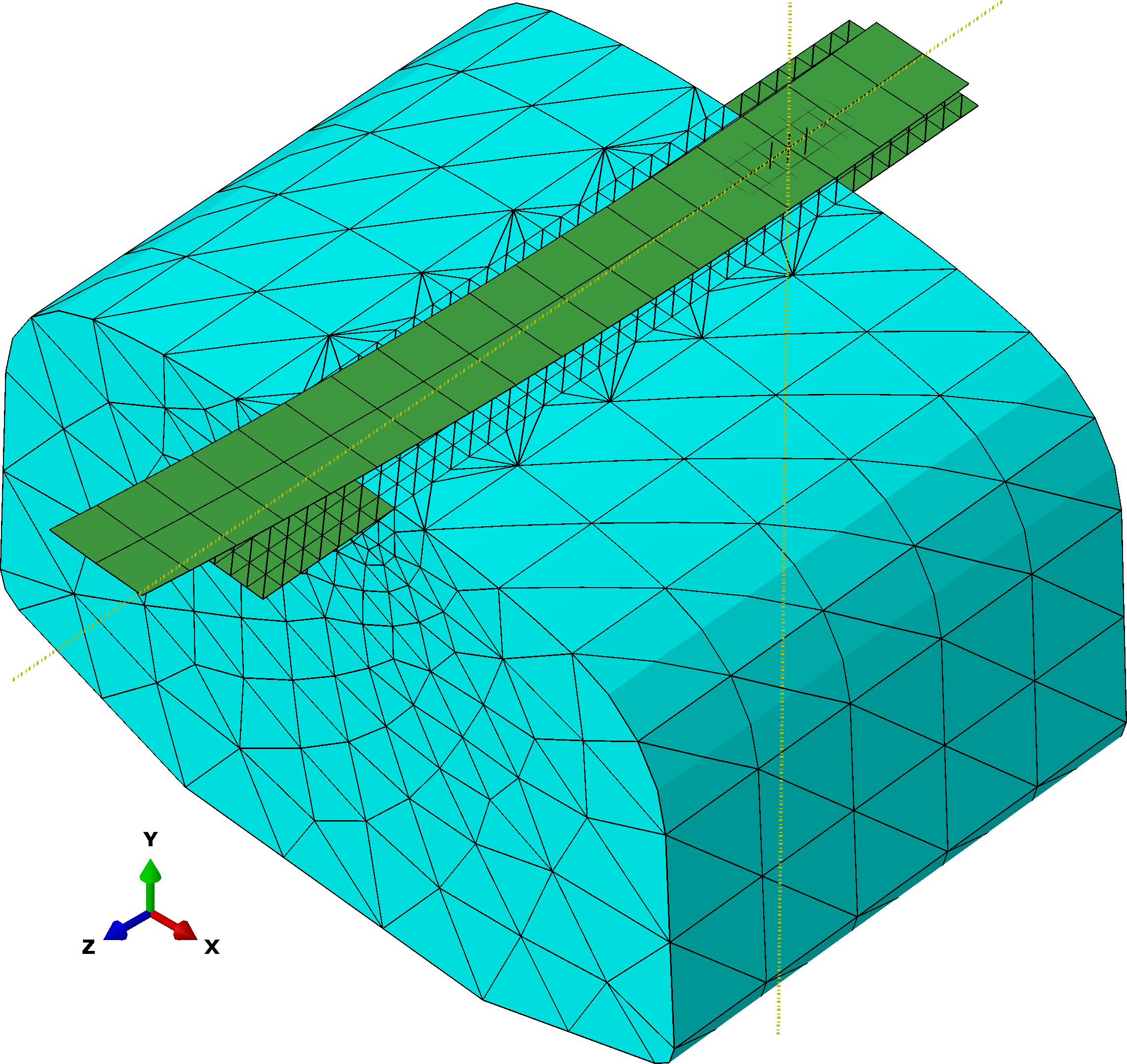
The form can be run with the default settings, except changing the paths to the generated rail_example.cae and folder wheel_example, or moving them to the default path specified. This action will create the following mesh, where the wheel is modeled using membrane elements.

The default settings do not add any field output. In that case, Abaqus’ default field outputs will be used. Note that this choice can result in very a large output database file (.odb) if many cycles are simulated.

rollover_mesh

Running the simulation from CAE¶

The standard user subroutine is added to the job, allowing to run the created job directly inside CAE. If running via the command line from a different folder (e.g. a computational cluster), please see Running simulation to ensure all required files are available. Using the command line is required if the input file was modified according to Adding rolling cycles.

Result¶

After successfully run with the default settings, the von Mises stresses in the rail at the middle of the rolling cycle become as shown here: rollover_result

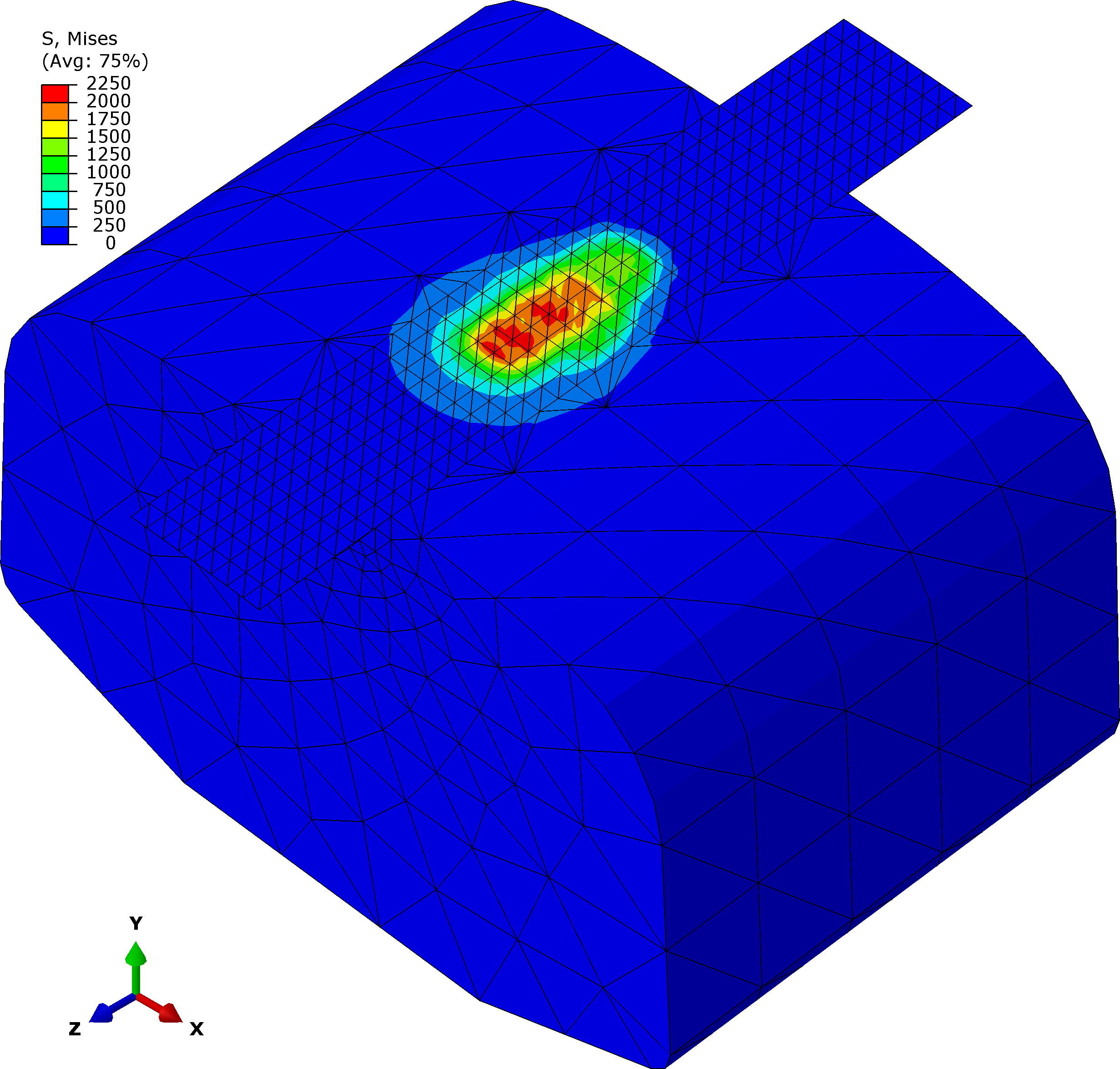
Note that the simulation time is rather long for this example, because the mesh on the rail has not been optimized. It is usually beneficial to use hexagonal elements.